Edit this page

From Training to Deployment with TensorFlow and OpenVINO

# @title Licensed under the Apache License, Version 2.0 (the "License");
# you may not use this file except in compliance with the License.
# You may obtain a copy of the License at
#
# https://www.apache.org/licenses/LICENSE-2.0
#
# Unless required by applicable law or agreed to in writing, software
# distributed under the License is distributed on an "AS IS" BASIS,
# WITHOUT WARRANTIES OR CONDITIONS OF ANY KIND, either express or implied.
# See the License for the specific language governing permissions and
# limitations under the License.

# Copyright 2018 The TensorFlow Authors
#
# Modified for OpenVINO Notebooks

This tutorial demonstrates how to train, convert, and deploy an image classification model with TensorFlow and OpenVINO. This particular notebook shows the process where we perform the inference step on the freshly trained model that is converted to OpenVINO IR with Model Optimizer. For faster inference speed on the model created in this notebook, check out the Post-Training Quantization with TensorFlow Classification Model notebook.

The training code is based on the official TensorFlow Image Classification Tutorial.

The flower_ir.bin and flower_ir.xml (pre-trained models) can be obtained by executing the code with ‘Runtime->Run All’ or the Ctrl+F9 command.

TensorFlow Image Classification Training

The first part of the tutorial shows how to classify images of flowers (based on the TensorFlow’s official tutorial). It creates an image classifier using a keras.Sequential model, and loads data using preprocessing.image_dataset_from_directory. You will gain practical experience with the following concepts:

• Efficiently loading a dataset off disk.

• Identifying overfitting and applying techniques to mitigate it, including data augmentation and Dropout.

This tutorial follows a basic machine learning workflow:

1. Examine and understand data

2. Build an input pipeline

3. Build the model

4. Train the model

5. Test the model

Import TensorFlow and Other Libraries

import os
import sys
from pathlib import Path

import PIL
import matplotlib.pyplot as plt
import numpy as np
import tensorflow as tf
from PIL import Image
from openvino.runtime import Core
from openvino.tools.mo import mo_tf
from tensorflow import keras
from tensorflow.keras import layers
from tensorflow.keras.models import Sequential

sys.path.append("../utils")
from notebook_utils import download_file

Download and Explore the Dataset

This tutorial uses a dataset of about 3,700 photos of flowers. The dataset contains 5 sub-directories, one per class:

flower_photo/
  daisy/
  dandelion/
  roses/
  sunflowers/
  tulips/

import pathlib
dataset_url = "https://storage.googleapis.com/download.tensorflow.org/example_images/flower_photos.tgz"
data_dir = tf.keras.utils.get_file('flower_photos', origin=dataset_url, untar=True)
data_dir = pathlib.Path(data_dir)

After downloading, you should now have a copy of the dataset available. There are 3,670 total images:

image_count = len(list(data_dir.glob('*/*.jpg')))
print(image_count)

3670

Here are some roses:

roses = list(data_dir.glob('roses/*'))
PIL.Image.open(str(roses[0]))

PIL.Image.open(str(roses[1]))

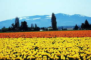
And some tulips:

tulips = list(data_dir.glob('tulips/*'))
PIL.Image.open(str(tulips[0]))

PIL.Image.open(str(tulips[1]))

Load Using keras.preprocessing

Let’s load these images off disk using the helpful image_dataset_from_directory utility. This will take you from a directory of images on disk to a tf.data.Dataset in just a couple lines of code. If you like, you can also write your own data loading code from scratch by visiting the load images tutorial.

Create a Dataset

Define some parameters for the loader:

batch_size = 32
img_height = 180
img_width = 180

It’s good practice to use a validation split when developing your model. Let’s use 80% of the images for training, and 20% for validation.

train_ds = tf.keras.preprocessing.image_dataset_from_directory(
  data_dir,
  validation_split=0.2,
  subset="training",
  seed=123,
  image_size=(img_height, img_width),
  batch_size=batch_size)

Found 3670 files belonging to 5 classes.
Using 2936 files for training.

val_ds = tf.keras.preprocessing.image_dataset_from_directory(
  data_dir,
  validation_split=0.2,
  subset="validation",
  seed=123,
  image_size=(img_height, img_width),
  batch_size=batch_size)

Found 3670 files belonging to 5 classes.
Using 734 files for validation.

You can find the class names in the class_names attribute on these datasets. These correspond to the directory names in alphabetical order.

class_names = train_ds.class_names
print(class_names)

['daisy', 'dandelion', 'roses', 'sunflowers', 'tulips']

Visualize the Data

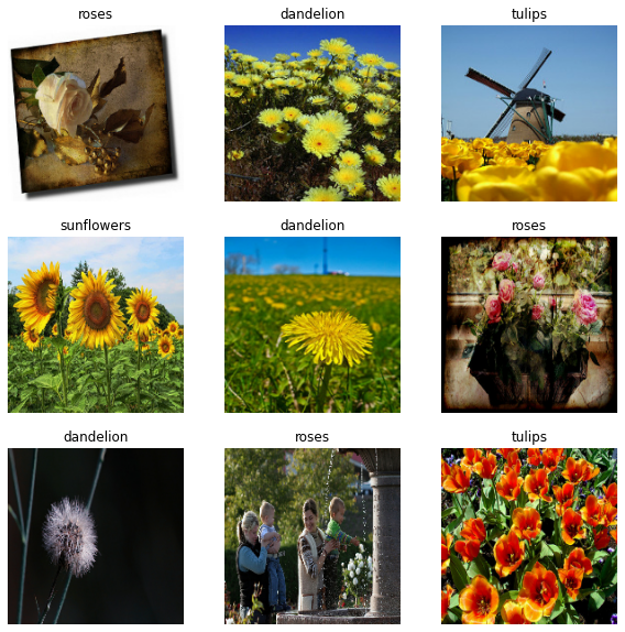
Here are the first 9 images from the training dataset.

plt.figure(figsize=(10, 10))
for images, labels in train_ds.take(1):
    for i in range(9):
        ax = plt.subplot(3, 3, i + 1)
        plt.imshow(images[i].numpy().astype("uint8"))
        plt.title(class_names[labels[i]])
        plt.axis("off")

You will train a model using these datasets by passing them to model.fit in a moment. If you like, you can also manually iterate over the dataset and retrieve batches of images:

for image_batch, labels_batch in train_ds:
    print(image_batch.shape)
    print(labels_batch.shape)
    break

(32, 180, 180, 3)
(32,)

The image_batch is a tensor of the shape (32, 180, 180, 3). This is a batch of 32 images of shape 180x180x3 (the last dimension refers to color channels RGB). The label_batch is a tensor of the shape (32,), these are corresponding labels to the 32 images.

You can call .numpy() on the image_batch and labels_batch tensors to convert them to a numpy.ndarray.

Configure the Dataset for Performance

Let’s make sure to use buffered prefetching so you can yield data from disk without having I/O become blocking. These are two important methods you should use when loading data.

Dataset.cache() keeps the images in memory after they’re loaded off disk during the first epoch. This will ensure the dataset does not become a bottleneck while training your model. If your dataset is too large to fit into memory, you can also use this method to create a performant on-disk cache.

Dataset.prefetch() overlaps data preprocessing and model execution while training.

Interested readers can learn more about both methods, as well as how to cache data to disk in the data performance guide.

# AUTOTUNE = tf.data.AUTOTUNE
AUTOTUNE = tf.data.experimental.AUTOTUNE
train_ds = train_ds.cache().shuffle(1000).prefetch(buffer_size=AUTOTUNE)
val_ds = val_ds.cache().prefetch(buffer_size=AUTOTUNE)

Standardize the Data

The RGB channel values are in the [0, 255] range. This is not ideal for a neural network; in general you should seek to make your input values small. Here, you will standardize values to be in the [0, 1] range by using a Rescaling layer.

normalization_layer = layers.experimental.preprocessing.Rescaling(1./255)

Note: The Keras Preprocessing utilities and layers introduced in this section are currently experimental and may change.

There are two ways to use this layer. You can apply it to the dataset by calling map:

normalized_ds = train_ds.map(lambda x, y: (normalization_layer(x), y))
image_batch, labels_batch = next(iter(normalized_ds))
first_image = image_batch[0]
# Notice the pixels values are now in `[0,1]`.
print(np.min(first_image), np.max(first_image))

0.0 0.9993465

Or, you can include the layer inside your model definition, which can simplify deployment. Let’s use the second approach here.

Note: you previously resized images using the image_size argument of image_dataset_from_directory. If you want to include the resizing logic in your model as well, you can use the Resizing layer.

Create the Model

The model consists of three convolution blocks with a max pool layer in each of them. There’s a fully connected layer with 128 units on top of it that is activated by a relu activation function. This model has not been tuned for high accuracy, the goal of this tutorial is to show a standard approach.

num_classes = 5

model = Sequential([
  layers.experimental.preprocessing.Rescaling(1./255, input_shape=(img_height, img_width, 3)),
  layers.Conv2D(16, 3, padding='same', activation='relu'),
  layers.MaxPooling2D(),
  layers.Conv2D(32, 3, padding='same', activation='relu'),
  layers.MaxPooling2D(),
  layers.Conv2D(64, 3, padding='same', activation='relu'),
  layers.MaxPooling2D(),
  layers.Flatten(),
  layers.Dense(128, activation='relu'),
  layers.Dense(num_classes)
])

Compile the Model

For this tutorial, choose the optimizers.Adam optimizer and losses.SparseCategoricalCrossentropy loss function. To view training and validation accuracy for each training epoch, pass the metrics argument.

model.compile(optimizer='adam',
              loss=tf.keras.losses.SparseCategoricalCrossentropy(from_logits=True),
              metrics=['accuracy'])

Model Summary

View all the layers of the network using the model’s summary method.

NOTE: This section is commented out for performance reasons. Please feel free to uncomment these to compare the results.

# model.summary()

Train the Model

# epochs=10
# history = model.fit(
#   train_ds,
#   validation_data=val_ds,
#   epochs=epochs
# )

Visualize Training Results

Create plots of loss and accuracy on the training and validation sets.

# acc = history.history['accuracy']
# val_acc = history.history['val_accuracy']

# loss = history.history['loss']
# val_loss = history.history['val_loss']

# epochs_range = range(epochs)

# plt.figure(figsize=(8, 8))
# plt.subplot(1, 2, 1)
# plt.plot(epochs_range, acc, label='Training Accuracy')
# plt.plot(epochs_range, val_acc, label='Validation Accuracy')
# plt.legend(loc='lower right')
# plt.title('Training and Validation Accuracy')

# plt.subplot(1, 2, 2)
# plt.plot(epochs_range, loss, label='Training Loss')
# plt.plot(epochs_range, val_loss, label='Validation Loss')
# plt.legend(loc='upper right')
# plt.title('Training and Validation Loss')
# plt.show()

As you can see from the plots, training accuracy and validation accuracy are off by large margin and the model has achieved only around 60% accuracy on the validation set.

Let’s look at what went wrong and try to increase the overall performance of the model.

Overfitting

In the plots above, the training accuracy is increasing linearly over time, whereas validation accuracy stalls around 60% in the training process. Also, the difference in accuracy between training and validation accuracy is noticeable — a sign of overfitting.

When there are a small number of training examples, the model sometimes learns from noises or unwanted details from training examples—to an extent that it negatively impacts the performance of the model on new examples. This phenomenon is known as overfitting. It means that the model will have a difficult time generalizing on a new dataset.

There are multiple ways to fight overfitting in the training process. In this tutorial, you’ll use data augmentation and add Dropout to your model.

Data Augmentation

Overfitting generally occurs when there are a small number of training examples. Data augmentation takes the approach of generating additional training data from your existing examples by augmenting them using random transformations that yield believable-looking images. This helps expose the model to more aspects of the data and generalize better.

You will implement data augmentation using the layers from tf.keras.layers.experimental.preprocessing. These can be included inside your model like other layers, and run on the GPU.

data_augmentation = keras.Sequential(
  [
    layers.experimental.preprocessing.RandomFlip("horizontal",
                                                 input_shape=(img_height,
                                                              img_width,
                                                              3)),
    layers.experimental.preprocessing.RandomRotation(0.1),
    layers.experimental.preprocessing.RandomZoom(0.1),
  ]
)

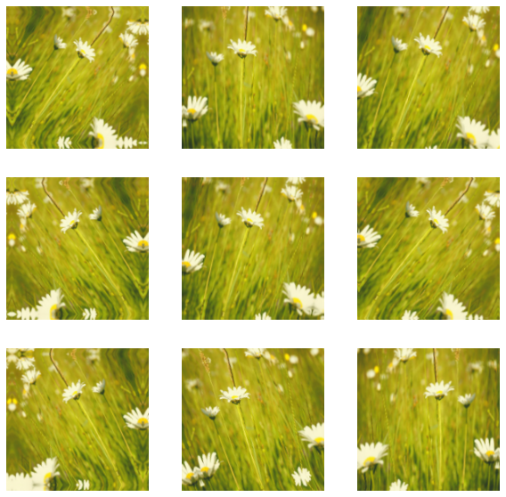
Let’s visualize what a few augmented examples look like by applying data augmentation to the same image several times:

plt.figure(figsize=(10, 10))
for images, _ in train_ds.take(1):
    for i in range(9):
        augmented_images = data_augmentation(images)
        ax = plt.subplot(3, 3, i + 1)
        plt.imshow(augmented_images[0].numpy().astype("uint8"))
        plt.axis("off")

You will use data augmentation to train a model in a moment.

Dropout

Another technique to reduce overfitting is to introduce Dropout to the network, a form of regularization.

When you apply Dropout to a layer it randomly drops out (by setting the activation to zero) a number of output units from the layer during the training process. Dropout takes a fractional number as its input value, in the form such as 0.1, 0.2, 0.4, etc. This means dropping out 10%, 20% or 40% of the output units randomly from the applied layer.

Let’s create a new neural network using layers.Dropout, then train it using augmented images.

model = Sequential([
  data_augmentation,
  layers.experimental.preprocessing.Rescaling(1./255),
  layers.Conv2D(16, 3, padding='same', activation='relu'),
  layers.MaxPooling2D(),
  layers.Conv2D(32, 3, padding='same', activation='relu'),
  layers.MaxPooling2D(),
  layers.Conv2D(64, 3, padding='same', activation='relu'),
  layers.MaxPooling2D(),
  layers.Dropout(0.2),
  layers.Flatten(),
  layers.Dense(128, activation='relu'),
  layers.Dense(num_classes)
])

Compile and Train the Model

model.compile(optimizer='adam',
              loss=tf.keras.losses.SparseCategoricalCrossentropy(from_logits=True),
              metrics=['accuracy'])

model.summary()

Model: "sequential_2"
_________________________________________________________________
Layer (type)                 Output Shape              Param #
=================================================================
sequential_1 (Sequential)    (None, 180, 180, 3)       0
_________________________________________________________________
rescaling_2 (Rescaling)      (None, 180, 180, 3)       0
_________________________________________________________________
conv2d_3 (Conv2D)            (None, 180, 180, 16)      448
_________________________________________________________________
max_pooling2d_3 (MaxPooling2 (None, 90, 90, 16)        0
_________________________________________________________________
conv2d_4 (Conv2D)            (None, 90, 90, 32)        4640
_________________________________________________________________
max_pooling2d_4 (MaxPooling2 (None, 45, 45, 32)        0
_________________________________________________________________
conv2d_5 (Conv2D)            (None, 45, 45, 64)        18496
_________________________________________________________________
max_pooling2d_5 (MaxPooling2 (None, 22, 22, 64)        0
_________________________________________________________________
dropout (Dropout)            (None, 22, 22, 64)        0
_________________________________________________________________
flatten_1 (Flatten)          (None, 30976)             0
_________________________________________________________________
dense_2 (Dense)              (None, 128)               3965056
_________________________________________________________________
dense_3 (Dense)              (None, 5)                 645
=================================================================
Total params: 3,989,285
Trainable params: 3,989,285
Non-trainable params: 0
_________________________________________________________________

epochs = 15
history = model.fit(
  train_ds,
  validation_data=val_ds,
  epochs=epochs
)

Epoch 1/15
92/92 [==============================] - 56s 599ms/step - loss: 1.4446 - accuracy: 0.3760 - val_loss: 1.1347 - val_accuracy: 0.5123
Epoch 2/15
92/92 [==============================] - 54s 589ms/step - loss: 1.1168 - accuracy: 0.5416 - val_loss: 1.0295 - val_accuracy: 0.5817
Epoch 3/15
92/92 [==============================] - 54s 588ms/step - loss: 1.0017 - accuracy: 0.6063 - val_loss: 0.9799 - val_accuracy: 0.6131
Epoch 4/15
92/92 [==============================] - 54s 590ms/step - loss: 0.9265 - accuracy: 0.6434 - val_loss: 0.9750 - val_accuracy: 0.5967
Epoch 5/15
92/92 [==============================] - 53s 581ms/step - loss: 0.8904 - accuracy: 0.6536 - val_loss: 0.9029 - val_accuracy: 0.6431
Epoch 6/15
92/92 [==============================] - 53s 581ms/step - loss: 0.8468 - accuracy: 0.6700 - val_loss: 0.9127 - val_accuracy: 0.6553
Epoch 7/15
92/92 [==============================] - 53s 579ms/step - loss: 0.8005 - accuracy: 0.6907 - val_loss: 0.8890 - val_accuracy: 0.6649
Epoch 8/15
92/92 [==============================] - 53s 578ms/step - loss: 0.7623 - accuracy: 0.7013 - val_loss: 0.8555 - val_accuracy: 0.6703
Epoch 9/15
92/92 [==============================] - 53s 577ms/step - loss: 0.7329 - accuracy: 0.7204 - val_loss: 0.8012 - val_accuracy: 0.6771
Epoch 10/15
92/92 [==============================] - 53s 578ms/step - loss: 0.7114 - accuracy: 0.7204 - val_loss: 0.8284 - val_accuracy: 0.6880
Epoch 11/15
92/92 [==============================] - 53s 580ms/step - loss: 0.6600 - accuracy: 0.7473 - val_loss: 0.7646 - val_accuracy: 0.6907
Epoch 12/15
92/92 [==============================] - 53s 579ms/step - loss: 0.6557 - accuracy: 0.7469 - val_loss: 0.8184 - val_accuracy: 0.7057
Epoch 13/15
92/92 [==============================] - 53s 580ms/step - loss: 0.6292 - accuracy: 0.7517 - val_loss: 0.7617 - val_accuracy: 0.7044
Epoch 14/15
92/92 [==============================] - 53s 580ms/step - loss: 0.5891 - accuracy: 0.7769 - val_loss: 0.7623 - val_accuracy: 0.7207
Epoch 15/15
92/92 [==============================] - 53s 579ms/step - loss: 0.5639 - accuracy: 0.7864 - val_loss: 0.7957 - val_accuracy: 0.6935

Visualize Training Results

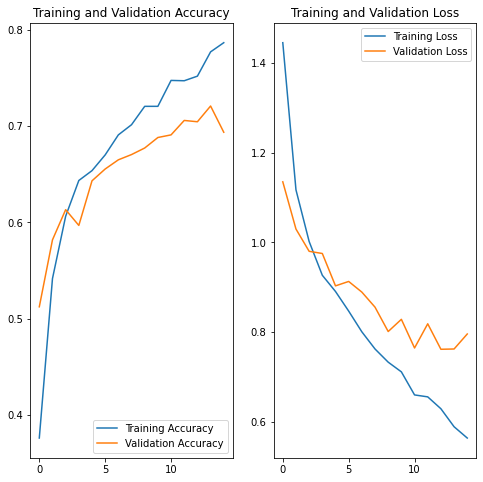
After applying data augmentation and Dropout, there is less overfitting than before, and training and validation accuracy are closer aligned.

acc = history.history['accuracy']
val_acc = history.history['val_accuracy']

loss = history.history['loss']
val_loss = history.history['val_loss']

epochs_range = range(epochs)

plt.figure(figsize=(8, 8))
plt.subplot(1, 2, 1)
plt.plot(epochs_range, acc, label='Training Accuracy')
plt.plot(epochs_range, val_acc, label='Validation Accuracy')
plt.legend(loc='lower right')
plt.title('Training and Validation Accuracy')

plt.subplot(1, 2, 2)
plt.plot(epochs_range, loss, label='Training Loss')
plt.plot(epochs_range, val_loss, label='Validation Loss')
plt.legend(loc='upper right')
plt.title('Training and Validation Loss')
plt.show()

Predict on New Data

Finally, let’s use our model to classify an image that wasn’t included in the training or validation sets.

Note: Data augmentation and Dropout layers are inactive at inference time.

sunflower_url = "https://storage.googleapis.com/download.tensorflow.org/example_images/592px-Red_sunflower.jpg"
sunflower_path = tf.keras.utils.get_file('Red_sunflower', origin=sunflower_url)

img = keras.preprocessing.image.load_img(
    sunflower_path, target_size=(img_height, img_width)
)
img_array = keras.preprocessing.image.img_to_array(img)
img_array = tf.expand_dims(img_array, 0)  # Create a batch

predictions = model.predict(img_array)
score = tf.nn.softmax(predictions[0])

print(
    "This image most likely belongs to {} with a {:.2f} percent confidence."
    .format(class_names[np.argmax(score)], 100 * np.max(score))
)

This image most likely belongs to sunflowers with a 99.76 percent confidence.

Save the TensorFlow Model

#save the trained model - a new folder flower will be created
#and the file "saved_model.pb" is the pre-trained model
model_dir = "model"
model_fname = f"{model_dir}/flower"
model.save(model_fname)

INFO:tensorflow:Assets written to: model/flower/assets

Convert the TensorFlow model with OpenVINO Model Optimizer

# The paths of the source and converted models
model_name = "flower"
model_path = Path(model_fname)
ir_data_type = "FP16"
ir_model_name = "flower_ir"

# Get the path to the Model Optimizer script

# Construct the command for Model Optimizer
mo_command = f"""mo
                 --saved_model_dir "{model_fname}"
                 --input_shape "[1,180,180,3]"
                 --data_type "{ir_data_type}"
                 --output_dir "{model_fname}"
                 --model_name "{ir_model_name}"
                 """
mo_command = " ".join(mo_command.split())
print("Model Optimizer command to convert TensorFlow to OpenVINO:")
print(mo_command)

Model Optimizer command to convert TensorFlow to OpenVINO:
mo --saved_model_dir "model/flower" --input_shape "[1,180,180,3]" --data_type "FP16" --output_dir "model/flower" --model_name "flower_ir"

# Run the Model Optimizer (overwrites the older model)
print("Exporting TensorFlow model to IR... This may take a few minutes.")
mo_result = %sx $mo_command
print("\n".join(mo_result))

Exporting TensorFlow model to IR... This may take a few minutes.
Model Optimizer arguments:
Common parameters:
    - Path to the Input Model:  None
    - Path for generated IR:    /home/runner/work/openvino_notebooks/openvino_notebooks/notebooks/301-tensorflow-training-openvino/model/flower
    - IR output name:   flower_ir
    - Log level:    ERROR
    - Batch:    Not specified, inherited from the model
    - Input layers:     Not specified, inherited from the model
    - Output layers:    Not specified, inherited from the model
    - Input shapes:     [1,180,180,3]
    - Source layout:    Not specified
    - Target layout:    Not specified
    - Layout:   Not specified
    - Mean values:  Not specified
    - Scale values:     Not specified
    - Scale factor:     Not specified
    - Precision of IR:  FP16
    - Enable fusing:    True
    - User transformations:     Not specified
    - Reverse input channels:   False
    - Enable IR generation for fixed input shape:   False
    - Use the transformations config file:  None
Advanced parameters:
    - Force the usage of legacy Frontend of Model Optimizer for model conversion into IR:   False
    - Force the usage of new Frontend of Model Optimizer for model conversion into IR:  False
TensorFlow specific parameters:
    - Input model in text protobuf format:  False
    - Path to model dump for TensorBoard:   None
    - List of shared libraries with TensorFlow custom layers implementation:    None
    - Update the configuration file with input/output node names:   None
    - Use configuration file used to generate the model with Object Detection API:  None
    - Use the config file:  None
OpenVINO runtime found in:  /opt/hostedtoolcache/Python/3.8.12/x64/lib/python3.8/site-packages/openvino
OpenVINO runtime version:   2022.1.0-7019-cdb9bec7210-releases/2022/1
Model Optimizer version:    2022.1.0-7019-cdb9bec7210-releases/2022/1
[ SUCCESS ] Generated IR version 11 model.
[ SUCCESS ] XML file: /home/runner/work/openvino_notebooks/openvino_notebooks/notebooks/301-tensorflow-training-openvino/model/flower/flower_ir.xml
[ SUCCESS ] BIN file: /home/runner/work/openvino_notebooks/openvino_notebooks/notebooks/301-tensorflow-training-openvino/model/flower/flower_ir.bin
[ SUCCESS ] Total execution time: 5.32 seconds.
[ SUCCESS ] Memory consumed: 582 MB.
It's been a while, check for a new version of Intel(R) Distribution of OpenVINO(TM) toolkit here https://software.intel.com/content/www/us/en/develop/tools/openvino-toolkit/download.html?cid=other&source=prod&campid=ww_2022_bu_IOTG_OpenVINO-2022-1&content=upg_all&medium=organic or on the GitHub*
[ INFO ] The model was converted to IR v11, the latest model format that corresponds to the source DL framework input/output format. While IR v11 is backwards compatible with OpenVINO Inference Engine API v1.0, please use API v2.0 (as of 2022.1) to take advantage of the latest improvements in IR v11.
Find more information about API v2.0 and IR v11 at https://docs.openvino.ai

Preprocessing Image Function

def pre_process_image(imagePath, img_height=180):
    # Model input format
    n, h, w, c = [1, img_height, img_height, 3]
    image = Image.open(imagePath)
    image = image.resize((h, w), resample=Image.BILINEAR)

    # Convert to array and change data layout from HWC to CHW
    image = np.array(image)
    input_image = image.reshape((n, h, w, c))

    return input_image

OpenVINO Inference Engine Setup

class_names=["daisy", "dandelion", "roses", "sunflowers", "tulips"]

model_xml = f"{model_fname}/flower_ir.xml"

# Load model
ie = Core()
model = ie.read_model(model=model_xml)

# Neural Compute Stick
# compiled_model = ie.compile_model(model=model, device_name="MYRIAD")
compiled_model = ie.compile_model(model=model, device_name="CPU")

del model

input_layer = compiled_model.input(0)
output_layer = compiled_model.output(0)

Run the Inference Step

# Run inference on the input image...
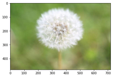
inp_img_url = "https://upload.wikimedia.org/wikipedia/commons/4/48/A_Close_Up_Photo_of_a_Dandelion.jpg"
OUTPUT_DIR = "output"
inp_file_name = f"A_Close_Up_Photo_of_a_Dandelion.jpg"
file_path = Path(OUTPUT_DIR)/Path(inp_file_name)

os.makedirs(OUTPUT_DIR, exist_ok=True)

# Download the image
download_file(inp_img_url, inp_file_name, directory=OUTPUT_DIR)

# Pre-process the image and get it ready for inference.
input_image = pre_process_image(file_path)

print(input_image.shape)
print(input_layer.shape)
res = compiled_model([input_image])[output_layer]

score = tf.nn.softmax(res[0])

# Show the results
image = Image.open(file_path)
plt.imshow(image)
print(
    "This image most likely belongs to {} with a {:.2f} percent confidence."
    .format(class_names[np.argmax(score)], 100 * np.max(score))
)

'output/A_Close_Up_Photo_of_a_Dandelion.jpg' already exists.
(1, 180, 180, 3)
{1, 180, 180, 3}
This image most likely belongs to dandelion with a 98.70 percent confidence.

<ipython-input-34-57303fd7ddec>:5: DeprecationWarning: BILINEAR is deprecated and will be removed in Pillow 10 (2023-07-01). Use Resampling.BILINEAR instead.
  image = image.resize((h, w), resample=Image.BILINEAR)

The Next Steps

This tutorial showed how to train a TensorFlow model, how to convert that model to OpenVINO’s IR format, and how to do inference on the converted model. For faster inference speed, you can quantize the IR model. To see how to quantize this model with OpenVINO’s Post-Training Optimization Tool, check out the Post-Training Quantization with TensorFlow Classification Model notebook.

Prev Next